← back to quantum computing
Superconducting Quantum Computing for Electrical Engineers
From Josephson Junctions to Qubit Readout: A Signal Processing Perspective
Hans Johnson
SQMS & Illinois Institute of Technology
Abstract
This document provides those with an electrical engineering background a comprehensive introduction to quantum computing, with emphasis on superconducting quantum computing, in the context of the RF and signal processing aspects that dominate practical implementations. The transmon qubit, the basis of quantum computation in the superconducting regime, is presented as a nonlinear LC oscillator; dispersive readout is explained as an RF measurement problem; and the signal processing challenges that limit current quantum computer performance are described. The treatment prioritizes intuition and EE analogies while providing mathematical foundations for readers seeking deeper understanding. A comprehensive survey of qubit modalities (superconducting, trapped ion, silicon spin, neutral atom, and photonic) compares performance metrics, infrastructure requirements, and fabrication approaches. Adaptive filtering techniques for qubit readout optimization are contextualized within the broader goal of fault-tolerant quantum computation.
1. Introduction: Why Should an Electrical Engineer Care About Quantum Computing?
Imagine running a Fast Fourier Transform on a dataset so large that classical computers would take longer than the age of the universe to complete it, yet a quantum computer could solve it in seconds. Imagine EDA tools that can optimize billion-transistor chip layouts by exploring all possible configurations simultaneously, rather than relying on heuristics. Imagine protein folding simulations that unlock CRISPR-based cancer therapies, or physics simulations that reveal new materials for room-temperature superconductors. These are not science fiction; they are the promises of fault-tolerant quantum computing, and they are closer than most people realize.
The catch? We are not there yet. Today's quantum computers are fragile, error-prone, and limited to a few hundred qubits. The path from laboratory curiosities to world-changing machines requires solving numerous engineering challenges, and many of these challenges are fundamentally electrical engineering problems: RF pulse generation with sub-nanosecond timing, cryogenic low-noise amplification at the quantum limit, high-speed digital signal processing for real-time error correction, and feedback control systems that operate faster than qubits can decohere. This is where EEs come in. The quantum computing revolution will not be led by physicists alone; it needs engineers who understand signal integrity, noise floors, and system integration. The field is wide open, and the opportunities for impact are immense.
The Core Insight for EEs: A superconducting qubit is essentially a nonlinear LC oscillator operating at microwave frequencies (~5 GHz) and cryogenic temperatures (~20 mK). The "quantum" behavior emerges from the circuit's nonlinearity, which creates uneven energy level spacing. Everything else (control, readout, error correction) is RF engineering and digital signal processing.
This document presents quantum computing from an EE perspective, translating quantum mechanical concepts into familiar circuit and signal processing terminology. The goal is to provide sufficient background for EE researchers to contribute meaningfully to quantum computing hardware development without requiring an extensive physics background.
1.1 The Quantum Computing Stack
A superconducting quantum computer consists of several layers, most of which involve traditional EE disciplines:
TABLE I: The Quantum Computing Stack
| Layer |
Function |
EE Discipline |
| Quantum Processor |
Josephson junctions at 20 mK |
Microwave circuit design, cryogenics |
| Control Electronics |
Precise microwave pulses |
RF/microwave engineering, DACs |
| Readout Chain |
Amplify/digitize signals |
Low-noise amplifiers, ADCs |
| Signal Processing |
State discrimination |
DSP, optimal filtering, ML |
| Real-time Control |
Feedback for QEC |
FPGA design, HDL |
This document focuses on the physics necessary to understand the signal processing layer, with particular attention to the readout discrimination problem.
1.2 Where Does Quantum Speedup Come From?
Before diving into hardware details, it is worth understanding why quantum computers can outperform classical computers for certain problems. The answer is subtle and often misunderstood.
1.2.1 The Naive (Wrong) Explanation
A common misconception is: "A qubit can be 0 and 1 simultaneously, so \(n\) qubits can represent \(2^n\) states at once, giving exponential parallelism." This is misleading because:
- While \(n\) qubits can exist in a superposition of \(2^n\) basis states, measurement only returns one outcome
- If superposition alone provided speedup, we could just flip \(n\) coins and call it parallel computation
- The speedup comes from something more subtle: interference
Why the Misconception Seems Plausible: The naive explanation feels right because quantum operations are linear. If you apply a function \(f\) to a superposition, you get the superposition of the outputs:
\(f(|0\rangle + |1\rangle) = f(|0\rangle) + f(|1\rangle)\)
This makes qubits look like "variables" in a program that can hold multiple values at once. If \(f\) is expensive to compute classically, it seems like we could evaluate it on all inputs in parallel. This is exactly what happens during the computation. The problem is that when we measure, we get one random output, not all of them. The "parallel computation" did happen, but we can only see one result. Without interference to bias which result we see, we have gained nothing over random guessing.
1.2.2 The Correct Explanation: Interference
Quantum algorithms exploit the wave-like nature of quantum states. In a superposition:
\[|\psi\rangle = \sum_{x=0}^{2^n-1} \alpha_x |x\rangle\]
(1)
Variable Definitions for Eq. (1):
\(|\psi\rangle\) — quantum state of \(n\) qubits
\(|x\rangle\) — computational basis state (e.g., \(|0101...\rangle\) representing binary number \(x\))
\(\alpha_x\) — complex amplitude for state \(|x\rangle\); probability of measuring \(x\) is \(|\alpha_x|^2\)
\(n\) — number of qubits; \(2^n\) possible basis states
the amplitudes \(\alpha_x\) are complex numbers that can interfere constructively or destructively when the quantum state evolves. A well-designed quantum algorithm:
- Prepares a superposition over all possible inputs (easy; a few Hadamard gates)
- Applies operations that encode the problem structure into the amplitudes
- Engineers interference so that "wrong" answers have amplitudes that cancel out, and "right" answers have amplitudes that add up
- Measures to obtain a right answer with high probability
EE Analogy: Think of a phased array antenna. Each element radiates in all directions (like a superposition), but the relative phases cause constructive interference in one direction and destructive interference in others. The array doesn't "try all directions at once"; it uses interference to concentrate energy where you want it. Quantum algorithms work similarly: they use interference to concentrate probability amplitude on correct answers.
Music Analogy: When two guitarists play the same note, the sound waves can reinforce each other (louder) or cancel out (quieter) depending on whether the waves are "in sync" or "out of sync." Quantum computers use this same wave-like behavior to make wrong answers cancel out and right answers get louder.
How Interference Is Engineered: The key insight is that quantum gates manipulate phases, not just probabilities. Consider a simple example with two paths to the same answer:
- Path A contributes amplitude \(+0.5\) to answer \(|x\rangle\)
- Path B contributes amplitude \(+0.5\) to answer \(|x\rangle\)
- Total amplitude: \(0.5 + 0.5 = 1.0\), so probability \(= |1.0|^2 = 1\) (certain)
Now consider a wrong answer where the phases differ:
- Path A contributes amplitude \(+0.5\) to answer \(|y\rangle\)
- Path B contributes amplitude \(-0.5\) to answer \(|y\rangle\)
- Total amplitude: \(0.5 + (-0.5) = 0\), so probability \(= |0|^2 = 0\) (impossible)
The algorithm designer's job is to construct a sequence of gates such that, after all operations complete, the wrong answers have uniformly distributed phases (they cancel when summed) while correct answers are in phase (they add constructively). This is not magic; it requires deep mathematical structure in the problem. Factoring integers has this structure; sorting a list does not.
Key Insight: Quantum speedup is not "trying all answers at once." It is carefully arranging phases so that computational paths leading to wrong answers destructively interfere while paths leading to correct answers constructively interfere. The algorithm must encode problem structure into phase relationships. Problems without exploitable structure do not benefit from quantum computation.
Seeing Interference in Action: For readers who want to visualize this process, interactive quantum circuit simulators provide immediate feedback:
- Quirk (https://algassert.com/quirk): Drag-and-drop circuit builder that shows amplitude magnitudes and phases in real time. Try building a 2-qubit Grover's algorithm to watch amplitudes redistribute.
- IBM Quantum Composer (https://quantum.ibm.com/composer): Build circuits and run them on real quantum hardware. Observe how measurement statistics match theoretical predictions.
1.2.3 Quantum Logic Gates: How Operations Work
Quantum algorithms are built from quantum gates, which transform qubit states. Unlike classical gates (AND, OR, NOT), quantum gates must be unitary: reversible and norm-preserving. This section introduces the essential gates.
Single-Qubit Gates: A single-qubit gate is a \(2 \times 2\) unitary matrix acting on the qubit state vector \([\alpha, \beta]^T\). The most important gates are:
- X Gate (NOT): Flips \(|0\rangle \leftrightarrow |1\rangle\). Matrix: \(X = \begin{pmatrix} 0 & 1 \\ 1 & 0 \end{pmatrix}\)
- Z Gate (Phase Flip): Leaves \(|0\rangle\) unchanged, flips the sign of \(|1\rangle\). Matrix: \(Z = \begin{pmatrix} 1 & 0 \\ 0 & -1 \end{pmatrix}\)
- Hadamard Gate (H): Creates superposition from basis states. \(H|0\rangle = \frac{1}{\sqrt{2}}(|0\rangle + |1\rangle)\), \(H|1\rangle = \frac{1}{\sqrt{2}}(|0\rangle - |1\rangle)\). Matrix: \(H = \frac{1}{\sqrt{2}}\begin{pmatrix} 1 & 1 \\ 1 & -1 \end{pmatrix}\)
On the Bloch sphere (Section 2), gates correspond to rotations: X rotates about the x-axis, Z rotates about the z-axis, and H rotates to the equator.
EE Analogy: Think of quantum gates as signal processing blocks with complex-valued transfer functions. The input is a 2D complex vector; the output is a transformed 2D complex vector. The unitarity constraint (\(U^\dagger U = I\)) is analogous to requiring a lossless, reversible transformation. This is like a passive reciprocal network: all information that goes in must come out.
Two-Qubit Gates and Entanglement: The CNOT (Controlled-NOT) gate is the essential two-qubit gate. It flips the "target" qubit if and only if the "control" qubit is \(|1\rangle\):
| Input |
Output |
| Control |
Target |
Control |
Target |
| \(|0\rangle\) | \(|0\rangle\) | \(|0\rangle\) | \(|0\rangle\) |
| \(|0\rangle\) | \(|1\rangle\) | \(|0\rangle\) | \(|1\rangle\) |
| \(|1\rangle\) | \(|0\rangle\) | \(|1\rangle\) | \(|1\rangle\) |
| \(|1\rangle\) | \(|1\rangle\) | \(|1\rangle\) | \(|0\rangle\) |
The CNOT gate creates entanglement when applied to a superposition. Starting from \(|00\rangle\):
- Apply H to qubit 1: \(H|0\rangle \otimes |0\rangle = \frac{1}{\sqrt{2}}(|0\rangle + |1\rangle) \otimes |0\rangle = \frac{1}{\sqrt{2}}(|00\rangle + |10\rangle)\)
- Apply CNOT (qubit 1 controls qubit 2): \(\frac{1}{\sqrt{2}}(|00\rangle + |11\rangle)\)
The result is a Bell state: the two qubits are correlated such that measuring one instantly determines the other, regardless of distance. This is not classical correlation (the qubits were not "secretly" in a definite state). Entanglement is a uniquely quantum resource exploited by algorithms and error correction.
Universal Gate Set: Any quantum computation can be built from just H, T (a phase gate), and CNOT. This is analogous to how any classical circuit can be built from NAND gates. In practice, quantum computers implement a small set of "native" gates efficiently, and compilers decompose arbitrary operations into these primitives.
1.2.4 Examples of Quantum Speedup
Well-known quantum algorithms and their speedups are summarized below. Each algorithm exploits a different type of mathematical structure.
TABLE II: Examples of Quantum Speedup
| Algorithm |
Problem |
Classical |
Quantum |
Speedup |
| Shor's [1] |
Factor integer \(N\) |
\(O(e^{n^{1/3}})\) |
\(O(n^3)\) |
Exponential |
| Grover's [2] |
Unsorted search |
\(O(N)\) |
\(O(\sqrt{N})\) |
Quadratic |
| Simulation |
Quantum systems |
\(O(2^n)\) |
\(O(\text{poly}(n))\) |
Exponential |
| HHL [3] |
Linear systems |
\(O(N)\) |
\(O(\log N)\) |
Exponential* |
*HHL speedup comes with significant caveats about input/output encoding.
What Each Algorithm Does:
Shor's Algorithm: Factors large integers by exploiting periodicity in modular exponentiation. This breaks RSA encryption, which relies on the difficulty of factoring products of large primes. A sufficiently large quantum computer could break most of today's public-key cryptography.
Grover's Algorithm: Searches an unsorted database of \(N\) items in \(O(\sqrt{N})\) time instead of \(O(N)\). This is "only" a quadratic speedup (not exponential), but it is provably optimal for unstructured search. It also applies to any NP problem: if verifying a solution takes time \(T\), Grover's can find one in \(O(\sqrt{N} \cdot T)\) time.
Quantum Simulation: Simulates quantum systems (molecules, materials, chemical reactions) efficiently. Classical computers struggle because simulating \(n\) quantum particles requires tracking \(2^n\) amplitudes. Quantum computers represent these states natively. Applications include drug discovery, materials science, and understanding high-temperature superconductivity.
HHL Algorithm: Solves systems of linear equations \(Ax = b\) exponentially faster than classical methods, with applications to machine learning and optimization. However, the speedup requires quantum-native input/output: preparing the input state and reading out the result both have overhead that can erase the advantage for many practical problems.
Important Caveat: Quantum computers do NOT speed up all problems. For most everyday computing tasks (web browsing, video encoding, databases), quantum computers offer no advantage. The speedup exists only for problems with specific mathematical structure that quantum interference can exploit.
1.2.5 What Quantum Computers Cannot Do
Quantum computers are not universal replacements for classical computers. Several fundamental limitations prevent QC from being "faster at everything":
- Measurement destroys information: After measurement, superposition collapses to a single outcome. You cannot extract all \(2^n\) computed values; you get one.
- No structure, no speedup: Quantum algorithms require mathematical structure (periodicity, symmetry, phase patterns) to engineer interference. Most problems lack this structure.
- Input/output bottleneck: Loading classical data into a quantum state and extracting results both require time proportional to data size. For problems dominated by I/O, quantum offers no advantage.
- Error correction overhead: Fault-tolerant quantum computing requires 100-1000 physical qubits per logical qubit. A "1000-qubit" quantum computer may have only 1-10 logical qubits.
TABLE III: Where Quantum Computing Helps vs. Does Not Help
| QC Provides Speedup |
QC Provides NO Speedup |
| Factoring large numbers (Shor's) |
Sorting, searching (only quadratic gain) |
| Simulating quantum systems |
General database queries |
| Certain optimization problems |
Video encoding/decoding |
| Breaking some cryptography (RSA, ECC) |
Web browsing, file I/O |
| Some machine learning tasks (limited) |
Most everyday computing |
| Quantum chemistry, drug discovery |
Compression algorithms |
Bottom Line: Quantum computers are specialized accelerators for problems with specific mathematical structure, not general-purpose replacements for classical computers. The laptop running your web browser will always be classical.
1.2.6 Why Readout Matters for Speedup
The interference patterns that encode the answer are fragile. They exist in the complex amplitudes \(\alpha_x\), which we cannot directly observe. We can only measure, which collapses the superposition and returns a single outcome. If the algorithm worked correctly, that outcome is (probably) the right answer. But there are failure modes:
- Decoherence during computation: If the coherence time T2 is too short (see Section 8 for formal definition), the interference pattern degrades before we finish the algorithm
- Gate errors: Imperfect gates corrupt the amplitudes, causing wrong answers to gain probability
- Readout errors: Even if the qubit is in the right state, misclassification reports the wrong answer
This is why high-fidelity readout is essential. The quantum computation may have produced the correct answer, but a readout error at the final step throws it away. For algorithms requiring many measurements (like variational algorithms), readout errors compound across shots. For quantum error correction, readout errors can be mistaken for data errors, triggering incorrect corrections.
Further Reading and Resources
For readers who want to explore quantum computing concepts in more depth before continuing with the hardware-focused sections of this document:
Video Lectures:
- "Quantum Computing for Computer Scientists" (Microsoft Research, YouTube): A rigorous 1-hour introduction that builds from linear algebra to Shor's algorithm.
Interactive Learning:
- IBM Quantum Learning (https://learning.quantum.ibm.com/): Structured courses from basics to advanced algorithms, with hands-on exercises on real quantum hardware.
- Qiskit Textbook (https://qiskit.org/textbook/): Comprehensive open-source textbook with executable Python code. Covers theory and implementation.
Deeper Reading:
- Scott Aaronson's blog (https://scottaaronson.blog/): A complexity theorist's perspective on quantum computing claims, hype, and genuine breakthroughs. Excellent for developing critical thinking about QC announcements.
2. The Transmon Qubit: A Nonlinear LC Oscillator
Quantum computation requires a physical system with exactly two accessible energy levels: a qubit. Why build one from an oscillator? Because quantum harmonic oscillators are among the best-understood quantum systems, they can be manufactured with existing microwave technology, and they couple naturally to electromagnetic control fields. The challenge is that a linear oscillator has infinitely many evenly-spaced energy levels, not two. The transmon solves this by introducing nonlinearity via a Josephson junction, creating unequal energy spacing that allows selective addressing of just the lowest two levels.
This section explains why linear oscillators fail as qubits, how the Josephson junction provides the necessary nonlinearity, and how the transmon circuit realizes a practical qubit. Understanding this circuit is essential for the readout discussion in later sections.
2.1 The Problem with Linear LC Circuits
Consider a standard LC oscillator. When quantized (treated quantum mechanically), its energy levels are:
\[E_n = \hbar\omega\left(n + \frac{1}{2}\right), \quad \omega = \frac{1}{\sqrt{LC}}\]
(2)
Variable Definitions for Eq. (2):
\(E_n\) — energy of the \(n\)-th quantum state (Joules)
\(\hbar = h/2\pi \approx 1.055 \times 10^{-34}\) J·s — reduced Planck constant
\(\omega\) — angular resonance frequency (rad/s)
\(n = 0, 1, 2, \ldots\) — quantum number (state index)
\(L, C\) — inductance and capacitance of the LC circuit
This is the quantum harmonic oscillator [8], with evenly spaced energy levels separated by \(\hbar\omega\). The transition frequency between any two adjacent levels is identical:
\[f_{01} = f_{12} = f_{23} = \cdots = \frac{\omega}{2\pi}\]
(3)
Variable Definitions for Eq. (3):
\(f_{01}, f_{12}, f_{23}, \ldots\) — transition frequencies between adjacent energy levels (Hz)
\(\omega\) — angular frequency of the oscillator (rad/s)
For a harmonic oscillator, all transition frequencies are identical.
The Problem: If all transitions have the same frequency, we cannot selectively drive just the \(|0\rangle\leftrightarrow|1\rangle\) transition. Any pulse that excites \(|0\rangle\rightarrow|1\rangle\) will also excite \(|1\rangle\rightarrow|2\rangle\), \(|2\rangle\rightarrow|3\rangle\), etc. We need a two-level system, but we have an infinite ladder.
2.2 The Josephson Junction Solution
The solution is to replace the linear inductor with a Josephson junction [4], which acts as a nonlinear inductor. The junction's inductance depends on the current flowing through it:
\[\boxed{L_J(\delta) = \frac{\Phi_0}{2\pi I_c \cos\delta}}\]
(4)
Variable Definitions:
\(\Phi_0 = h/2e \approx 2.07 \times 10^{-15}\) Wb — magnetic flux quantum
\(I_c\) — critical current of the junction (typically ~10-100 nA)
\(\delta = \phi_L - \phi_R\) — superconducting phase difference across the junction
EE Analogy: Think of the Josephson junction as a varactor (voltage-dependent capacitor), but for inductance. Just as a varactor's capacitance varies with bias voltage, the Josephson junction's inductance varies with the current (or equivalently, the phase) across it.
This nonlinear inductance creates a cosine potential instead of the quadratic potential of a linear inductor. The energy stored in the junction is:
\[U_J = -E_J \cos\delta, \quad \text{where } E_J = \frac{\Phi_0 I_c}{2\pi}\]
(5)
Variable Definitions for Eq. (5):
\(U_J\) — potential energy stored in the Josephson junction (Joules)
\(E_J\) — Josephson energy (Joules); sets the depth of the cosine potential well
\(\delta\) — superconducting phase difference across the junction (radians)
\(\Phi_0 = h/2e \approx 2.07 \times 10^{-15}\) Wb — magnetic flux quantum
\(I_c\) — critical current of the junction (Amperes)
The cosine potential has a different curvature than a parabola, leading to unequally spaced energy levels:
\[\boxed{f_{12} = f_{01} - \alpha, \quad \alpha \approx \frac{E_C}{h} \approx 200\text{-}300 \text{ MHz}}\]
(6)
Variable Definitions for Eq. (6):
\(f_{01}\) — transition frequency between ground state \(|0\rangle\) and first excited state \(|1\rangle\) (Hz)
\(f_{12}\) — transition frequency between \(|1\rangle\) and \(|2\rangle\) (Hz)
\(\alpha\) — anharmonicity; the frequency difference that enables selective addressing
\(E_C = e^2/(2C)\) — charging energy of the qubit capacitance (Joules)
\(h \approx 6.63 \times 10^{-34}\) J·s — Planck constant
The parameter \(\alpha\) is called the anharmonicity [10]. It represents the frequency difference between adjacent transitions. With \(\alpha \approx 200\) MHz, we can send a ~20 ns pulse (bandwidth ~50 MHz) that drives \(|0\rangle\leftrightarrow|1\rangle\) without significantly exciting \(|1\rangle\rightarrow|2\rangle\).
2.3 The Transmon Circuit
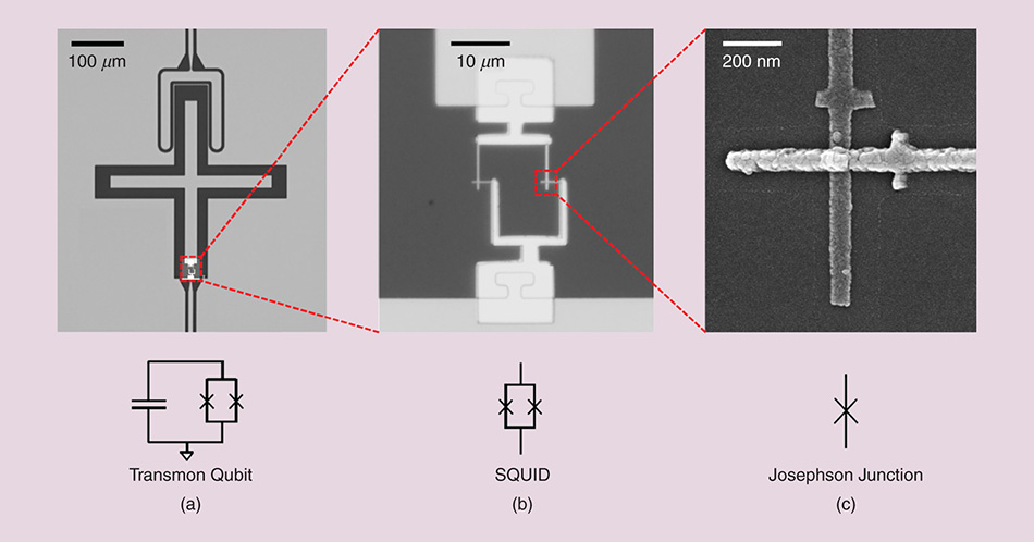
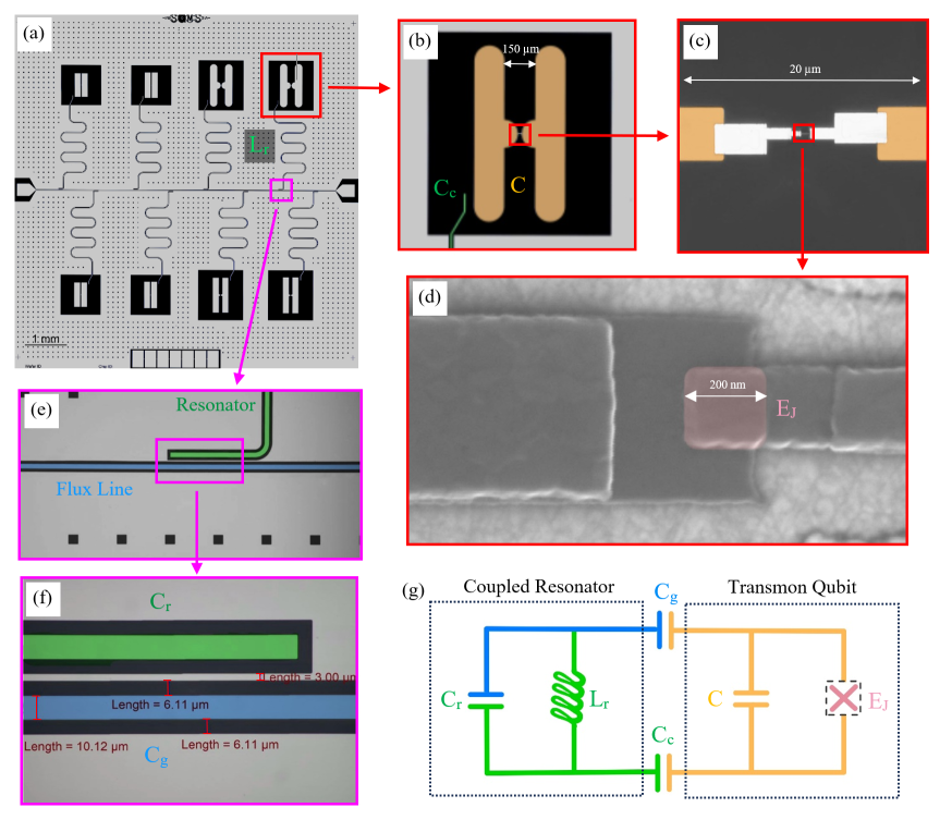
The transmon [10] (transmission-line shunted plasma oscillation qubit) is the most common superconducting qubit design. At its core, it consists of a Josephson junction shunted by a large capacitor—but physical implementations reveal a rich hierarchical structure spanning three orders of magnitude in scale.
Modern transmons typically use a SQUID (Superconducting Quantum Interference Device)—two Josephson junctions in a superconducting loop—rather than a single junction. This allows in-situ tuning of the effective Josephson energy via an external magnetic flux threading the loop. The large cross-shaped pads visible in panel (a) form the shunt capacitor \(C_s\); their geometry is carefully designed to minimize surface losses while providing the required capacitance (~80 fF) for operation in the transmon regime.
TABLE IV: Transmon Qubit Parameters
| Parameter |
Typical Value |
Derived Quantity |
| Shunt capacitance \(C_s\) |
~80 fF |
\(E_C/h \approx 240\) MHz |
| Critical current \(I_c\) |
~40 nA |
\(E_J/h \approx 20\) GHz |
| Josephson inductance \(L_{J0}\) |
~8 nH |
At zero bias |
| Qubit frequency \(f_{01}\) |
4-5 GHz |
\(\approx \sqrt{8E_JE_C}/h\) |
| Anharmonicity \(\alpha\) |
200-300 MHz |
\(\approx E_C/h\) |
Key Insight: The transmon operates in the regime \(E_J \gg E_C\)
[10] (typically \(E_J/E_C \approx 50\text{-}100\)). This makes the qubit insensitive to charge noise (a major source of decoherence in earlier designs) while maintaining sufficient anharmonicity for selective addressing.
Physical Architecture Details:
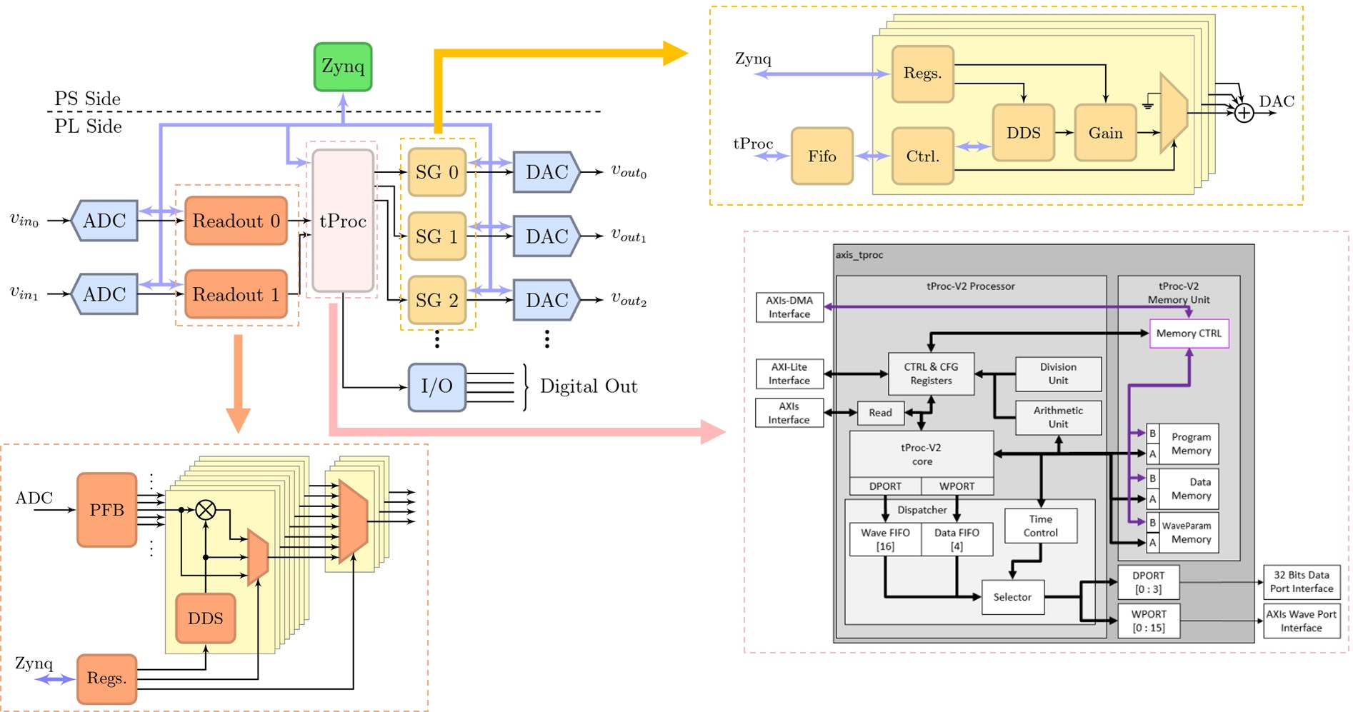
The chip in Fig. 2(a) contains eight qubits arranged to test different capacitor geometries. Each qubit is coupled to a coplanar waveguide (CPW) resonator, visible as the meandering transmission line in panel (e), which serves as the primary interface for both control and readout.
50 Ω Launchers and Chip I/O: The rectangular pads at the left and right sides of the chip are 50 Ω launchers: impedance-matched transitions that connect the on-chip transmission lines to external microwave electronics. Gold or aluminum wirebonds connect these launchers to a printed circuit board (PCB) mounted in the cryostat. The 50 Ω characteristic impedance matches standard microwave test equipment, which minimizes signal reflections that would otherwise distort pulses and corrupt readout signals.
Feedline Architecture and Frequency Multiplexing: A central feedline (visible running horizontally across the chip) acts as a shared microwave highway. Multiple readout resonators, each tuned to a different frequency, couple capacitively to this feedline. This architecture enables frequency-division multiplexing: a single input/output line can address many qubits simultaneously by sending microwave tones at each resonator's unique frequency. Adjacent resonators are typically spaced 50-100 MHz apart to prevent crosstalk [12].
Qubit-Resonator Coupling: Each qubit couples to its dedicated resonator through a small coupling capacitor \(C_g\). The coupling strength \(g/2\pi \sim 50\text{-}100\) MHz is carefully engineered: strong enough for fast readout, but weak enough to operate in the dispersive regime where the qubit-resonator detuning \(\Delta = \omega_q - \omega_r\) satisfies \(|\Delta| \gg g\).
Signal Flow:
Readout: A microwave tone near the resonator frequency enters through one launcher, travels along the feedline, and interacts with each resonator it passes. The transmitted (or reflected) signal carries phase and amplitude information encoding the qubit states, then exits through the opposite launcher to be amplified and digitized.
Control: Qubit drive pulses at the qubit frequency \(f_{01}\) also enter through the feedline. Although primarily intended for readout, the resonator acts as a bandpass filter that couples control pulses to the qubit while providing Purcell filtering, which suppresses qubit energy decay into the feedline at frequencies far from the resonator.
Materials Engineering: Achieving long coherence times requires careful materials selection. The SQMS design uses:
- Sapphire substrate: Low-loss dielectric (\(\tan\delta < 10^{-6}\)) with excellent thermal conductivity at millikelvin temperatures
- Niobium-tantalum encapsulation: Protects niobium surfaces from native oxide formation, reducing two-level system (TLS) defects that limit \(T_1\) [27]
- Aluminum Josephson junctions: Standard Al/AlO\(_x\)/Al trilayer fabricated via double-angle evaporation, with junction area ~200 nm × 200 nm setting \(E_J\)
3. Cooper Pairs and the Josephson Effect
This section explains the physics underlying the Josephson junction. For readers primarily interested in signal processing applications, this section can be skimmed; the key result is Equation (4).
3.1 Why Superconductors Are Different
At temperatures below the critical temperature \(T_c\) (about 1.2 K for aluminum) [6], electrons in a metal form bound pairs called Cooper pairs [5]. This pairing is mediated by phonons (lattice vibrations):
- An electron moving through the lattice attracts nearby positive ions
- This creates a region of slightly higher positive charge density
- A second electron is attracted to this region
- The two electrons become weakly bound (binding energy ~0.1-1 meV)
TABLE V: Single Electron vs. Cooper Pair Properties
| Property |
Single Electron |
Cooper Pair |
| Spin | 1/2 (fermion) | 0 (boson) |
| Pauli exclusion | Yes | No |
| Charge | \(-e\) | \(-2e\) |
| Can occupy same state | No | Yes (all pairs) |
The key difference is that Cooper pairs are bosons. Because bosons are not subject to the Pauli exclusion principle, they can all condense into the same quantum ground state [6]. This Bose-Einstein condensate is described by a single macroscopic wavefunction:
\[\Psi = \sqrt{n_s} \cdot e^{i\phi}\]
(7)
Variable Definitions for Eq. (7):
\(\Psi\) — macroscopic wavefunction of the superconducting condensate
\(n_s\) — Cooper pair density (pairs per unit volume)
\(\phi\) — macroscopic phase of the superconductor (radians); coherent across the entire material
\(|\Psi|^2 = n_s\) — the squared magnitude gives the pair density
EE Analogy: Think of the phase \(\phi\) as a clock signal that is perfectly synchronized across the entire superconductor. All Cooper pairs oscillate in phase, like a distributed oscillator with zero phase noise.
Music Analogy: Imagine a massive choir where every singer holds the exact same note in perfect unison, with no one drifting sharp or flat. Cooper pairs in a superconductor are like this choir: millions of electron pairs all "singing" at exactly the same phase, which is why current flows without resistance.
3.2 Quantum Tunneling
Quantum tunneling [8] is not unique to Cooper pairs; it occurs for any quantum particle. The key physics is that a particle's wavefunction does not stop at a potential barrier but decays exponentially inside it:
\[\psi(x) \propto e^{-\kappa x}, \quad \kappa = \frac{\sqrt{2m(V_0-E)}}{\hbar}\]
(8)
Variable Definitions for Eq. (8):
\(\psi(x)\) — particle wavefunction amplitude inside the barrier
\(\kappa\) — decay constant inside the barrier (inverse meters)
\(m\) — particle mass (kg)
\(V_0\) — barrier height (Joules)
\(E\) — particle energy (Joules); must have \(E < V_0\) for tunneling
\(x\) — position inside the barrier (meters)
If the barrier is thin enough (~1 nm for a Josephson junction), the wavefunction has non-zero amplitude on the other side, giving a finite tunneling probability:
\[T \approx e^{-2\kappa d}\]
(9)
Variable Definitions for Eq. (9):
\(T\) — tunneling probability (dimensionless, 0 to 1)
\(\kappa\) — decay constant inside the barrier (m\(^{-1}\))
\(d\) — barrier thickness (meters)
For a Josephson junction with ~1 nm oxide barrier, \(T\) can be significant (~0.01-0.1).
Single electrons tunnel through thin insulators routinely (this is how scanning tunneling microscopes and flash memory work). What makes Josephson tunneling special is that Cooper pairs tunnel coherently (preserving phase information) and dissipationlessly (no energy loss).
3.3 The Josephson Equations
When two superconductors are separated by a thin insulator, Cooper pairs can tunnel between them [4]. The tunneling current depends on the phase difference \(\delta = \phi_L - \phi_R\):
\[\boxed{I = I_c \sin\delta} \quad \text{(First Josephson Equation)}\]
(10)
Variable Definitions for Eq. (10):
\(I\) — supercurrent flowing through the junction (Amperes)
\(I_c\) — critical current; maximum supercurrent the junction can carry (Amperes)
\(\delta = \phi_L - \phi_R\) — phase difference between left and right superconductors (radians)
The phase evolves according to the voltage across the junction:
\[\boxed{\frac{d\delta}{dt} = \frac{2eV}{\hbar} = \frac{2\pi V}{\Phi_0}} \quad \text{(Second Josephson Equation)}\]
(11)
Variable Definitions for Eq. (11):
\(d\delta/dt\) — rate of change of phase difference (rad/s)
\(V\) — voltage across the junction (Volts)
\(e \approx 1.602 \times 10^{-19}\) C — electron charge
\(\Phi_0 = h/2e \approx 2.07 \times 10^{-15}\) Wb — magnetic flux quantum
Note: A DC voltage causes the phase to wind continuously, producing an AC current at frequency \(f = V/\Phi_0\).
3.4 Why Josephson Tunneling is Dissipationless
In a superconductor, there is an energy gap \(\Delta\) (~0.2 meV for aluminum). To create a quasiparticle excitation (break a Cooper pair), energy \(2\Delta\) is required. For voltages \(V < 2\Delta/e \approx 0.4\) mV:
- Not enough energy to break Cooper pairs
- No quasiparticle current (which would be dissipative)
- Only coherent Cooper pair tunneling occurs
- Zero resistance (supercurrent)
Qubits always operate in this sub-gap regime, ensuring dissipationless dynamics.
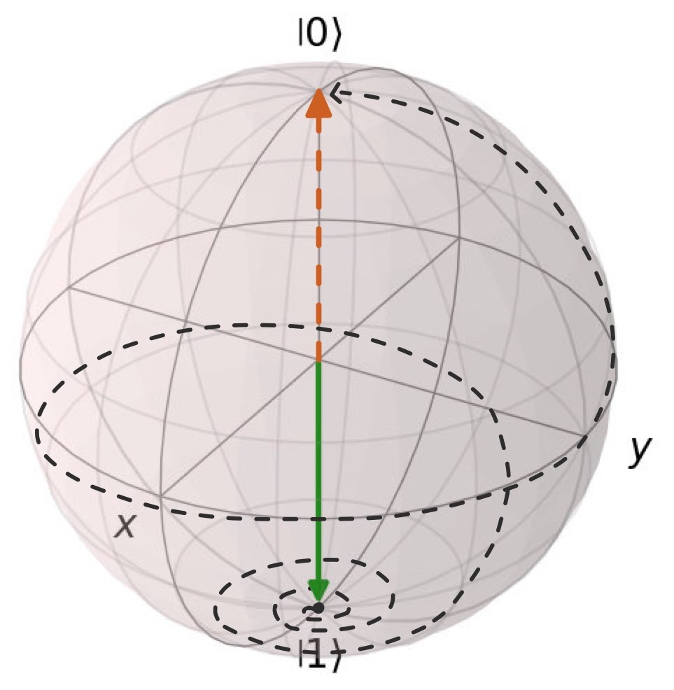
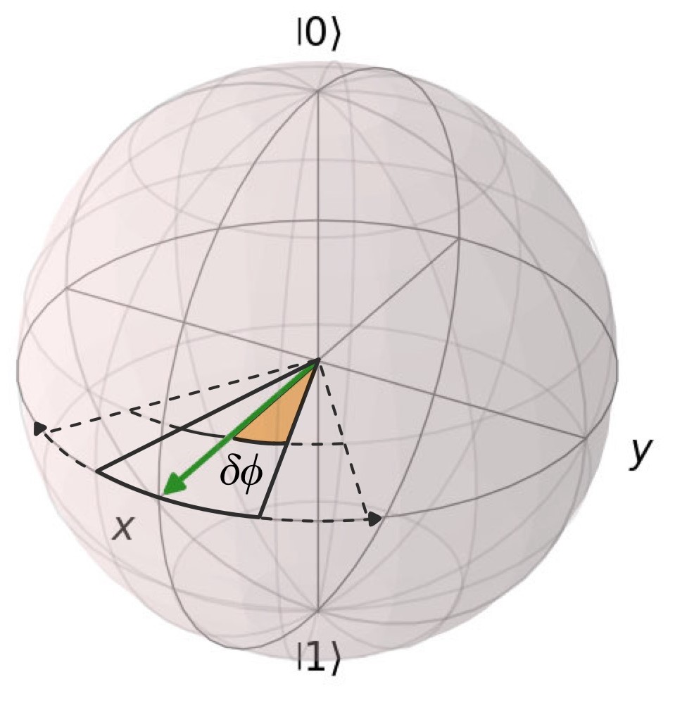
3.5 Visualizing Qubit States: Bloch Sphere and Wigner Function
Before moving to measurement, it is worth briefly noting how qubit states are typically visualized.
The Bloch Sphere: Any pure state of a two-level quantum system (qubit) can be written as:
\[|\psi\rangle = \cos\left(\frac{\theta}{2}\right)|0\rangle + e^{i\phi}\sin\left(\frac{\theta}{2}\right)|1\rangle\]
(12)
Variable Definitions for Eq. (12):
\(\theta\) — polar angle from the z-axis (0 to \(\pi\))
\(\phi\) — azimuthal angle in the x-y plane (0 to \(2\pi\))
\(|0\rangle, |1\rangle\) — computational basis states
This parameterization maps qubit states to points on a unit sphere called the Bloch sphere [7]. The north pole represents \(|0\rangle\), the south pole represents \(|1\rangle\), and points on the equator represent equal superpositions with different phases.
EE Analogy: The Bloch sphere is a 3D extension of a phasor diagram. The z-axis represents the "amplitude" (population difference between \(|0\rangle\) and \(|1\rangle\)), while the azimuthal angle represents phase, just as in a phasor.
The Wigner Function: The Wigner function \(W(x, p)\) is a quasi-probability distribution that represents quantum states in phase space. Unlike classical probability distributions, the Wigner function can take negative values, which is a signature of non-classical behavior.
EE Analogy: If you know the Wigner-Ville distribution from signal processing, the quantum Wigner function is its direct analog. Both are phase space representations, and both can exhibit negative values due to interference between components.
Why Wigner Negativity Matters in Quantum Computing:
- Hudson's Theorem: A pure quantum state has a non-negative Wigner function if and only if it is Gaussian. Any non-Gaussian state must have negative regions.
- Quantum vs. Classical: A positive Wigner function can be interpreted as a classical probability distribution. Negativity proves that no such classical description exists.
- Computational Resource: In bosonic quantum computing, Wigner negativity is a resource for quantum advantage.
TABLE VI: When to Use Each Quantum State Representation
| Representation |
Best For |
Limitations |
| Bloch Sphere |
Single-qubit gates, visualizing rotations, understanding pulse sequences |
Only works for single qubits; does not capture entanglement |
| Wigner Function |
Cavity states, bosonic codes, visualizing non-classical features |
Requires 2D plotting; less intuitive for simple qubit operations |
| IQ Plane (Readout) |
Measurement discrimination, signal processing, classifier design |
Classical representation; does not capture quantum coherence |
4. Qubit State Measurement: Dispersive Readout
Measuring a qubit state is fundamentally an RF engineering problem. This section describes the standard approach used in nearly all superconducting quantum computers.
4.1 The Dispersive Regime
The qubit is capacitively coupled to a readout resonator (a linear microwave cavity, typically ~7 GHz). When the qubit and resonator frequencies are far detuned (\(|\omega_q - \omega_r| \gg g\), where \(g\) is the coupling strength), the system is in the dispersive regime [9,12].
In this regime, the resonator frequency depends on the qubit state:
\[\boxed{f_r^{|0\rangle} = f_r + \chi, \quad f_r^{|1\rangle} = f_r - \chi}\]
(13)
Variable Definitions for Eq. (13):
\(f_r\) — bare resonator frequency (~7 GHz)
\(\chi\) — dispersive shift (typically 1-5 MHz)
The total shift between states is \(2\chi\)
EE Analogy: This is analogous to a voltage-controlled oscillator (VCO) where the "control voltage" is the qubit state. The qubit acts as a state-dependent reactive load that pulls the resonator frequency.
Music Analogy: Imagine gently touching a vibrating guitar string. Depending on where you touch it, the pitch shifts slightly. In dispersive readout, we "listen" to a resonator's pitch to figure out the qubit's state.
Intuitive Picture (Interference Again): The dispersive shift can be understood as interference, connecting back to Section 1. The qubit and resonator exchange virtual photons: the resonator briefly "lends" energy to the qubit, which returns it. Depending on the qubit state, these exchanges create constructive interference at slightly different frequencies.
4.2 The Measurement Process
To measure the qubit, we probe the resonator with a microwave tone and detect the state-dependent phase/amplitude shift:
- Send probe tone at frequency near \(f_r\)
- Signal reflects off resonator with state-dependent phase:
- Qubit in \(|0\rangle\): resonator at \(f_r + \chi\) → phase \(\phi_0\)
- Qubit in \(|1\rangle\): resonator at \(f_r - \chi\) → phase \(\phi_1\)
- Amplify using cryogenic amplifier (HEMT or JPA/TWPA)
- Downconvert to intermediate frequency (~100 MHz)
- Digitize I and Q quadratures
- Classify in IQ plane to determine state
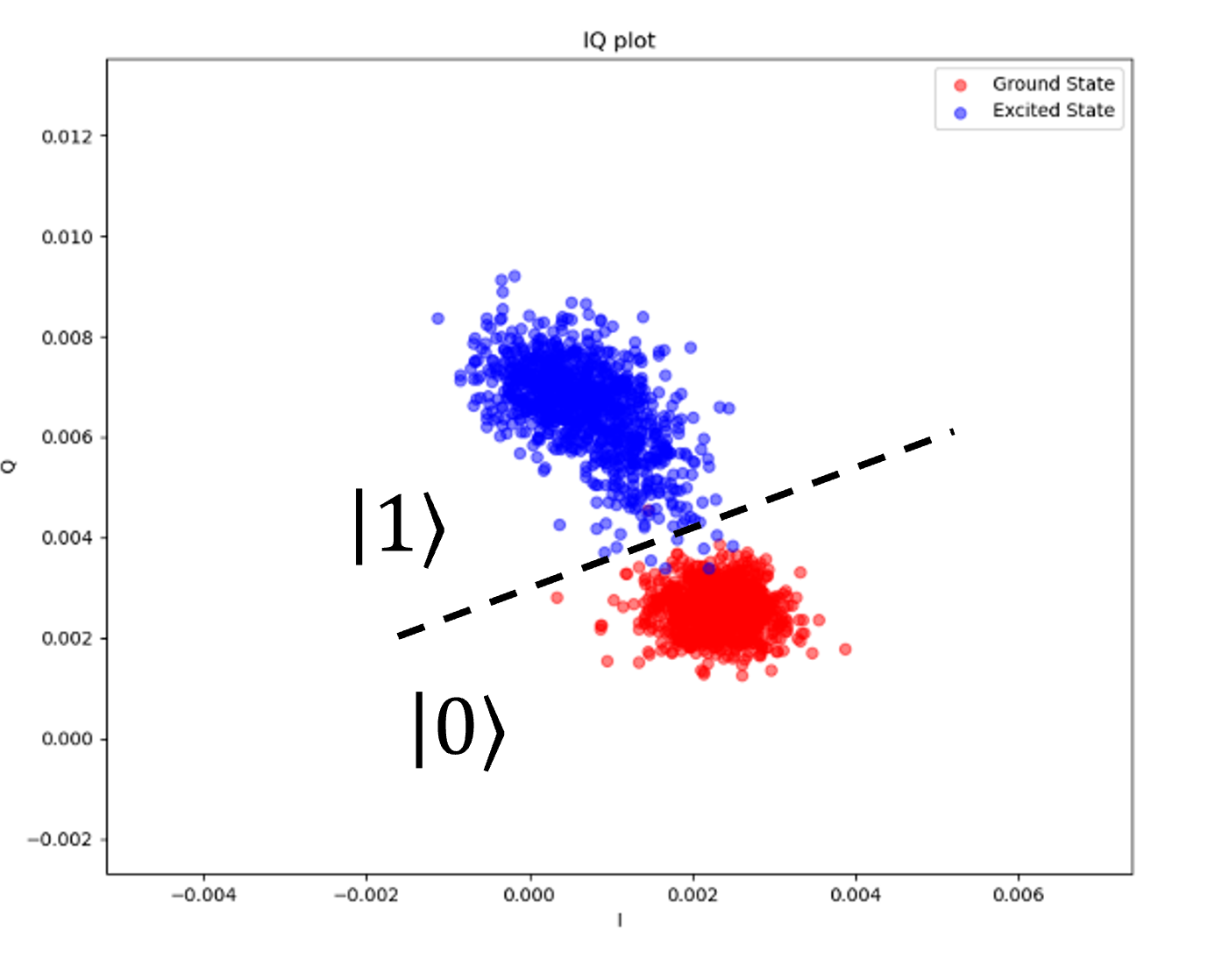
4.3 The IQ Plane Representation
After digitization, each readout pulse produces a point in the IQ plane. Due to the dispersive shift, \(|0\rangle\) and \(|1\rangle\) states produce points clustered in different regions.
What the Clusters Tell Us:
- Cluster separation is proportional to the dispersive shift \(\chi\) and integration time \(\tau\). The total separation scales as \(2\chi\tau\).
- Cluster width reflects the total system noise, combining thermal fluctuations, amplifier noise, and any other broadening mechanisms.
The signal-to-noise ratio for state discrimination is simply:
\[\text{SNR} = \frac{\text{cluster separation}}{\text{cluster width}}\]
Key Insight: The readout problem is fundamentally a two-class Gaussian classification problem in 2D. The clusters overlap due to noise; classification errors occur when a point from one class falls in the other class's region. Improving SNR directly improves classification fidelity.
4.4 Sources of Readout Error
TABLE VII: Sources of Readout Error
| Error Source |
Mechanism |
Typical Contribution |
| Thermal noise |
Johnson noise from finite temperature |
Negligible at 20 mK |
| Amplifier noise |
Added noise from HEMT (~2-10 K noise temp) |
Dominant for most systems |
| Qubit decay (T1) |
\(|1\rangle\rightarrow|0\rangle\) decay during measurement |
Grows with readout time |
| State preparation |
Qubit not in intended initial state |
~0.5-2% |
| Measurement-induced |
High photon number kicks qubit to \(|2\rangle\) |
Limits max readout power |
The fundamental tradeoff is between integration time and T1 decay:
- Longer integration → more signal → higher SNR
- But longer integration → more time for \(|1\rangle\rightarrow|0\rangle\) decay → measure wrong state
- Optimal readout time is typically 100-500 ns
4.5 From Superposition to Definite Outcomes: How Measurement Works
A fundamental question arises: if a qubit can exist in a superposition of \(|0\rangle\) and \(|1\rangle\), how do we ever get a definite answer?
The Measurement Postulate: In quantum mechanics, measurement is fundamentally different from classical observation [7]. When we measure a qubit in the state:
\[|\psi\rangle = \alpha|0\rangle + \beta|1\rangle, \quad |\alpha|^2 + |\beta|^2 = 1\]
(14)
Variable Definitions for Eq. (14):
\(|\psi\rangle\) — quantum state of the qubit
\(|0\rangle, |1\rangle\) — computational basis states (ground and excited states)
\(\alpha, \beta\) — complex probability amplitudes
\(|\alpha|^2\) — probability of measuring state \(|0\rangle\)
\(|\beta|^2\) — probability of measuring state \(|1\rangle\)
The measurement does not reveal "a little bit of \(|0\rangle\) and a little bit of \(|1\rangle\)." Instead:
- We get exactly \(|0\rangle\) with probability \(|\alpha|^2\)
- We get exactly \(|1\rangle\) with probability \(|\beta|^2\)
- The superposition is destroyed (this is called "wavefunction collapse")
- After measurement, the qubit is in whichever state we measured
EE Analogy: Think of measurement like sampling a noisy signal with a 1-bit ADC. Before sampling, the signal could be anywhere. After sampling, you get either 0 or 1. The "superposition" is like the continuous voltage; the "measurement" is the quantization. The key difference: in quantum mechanics, this discretization is fundamental, not due to limited resolution.
Music Analogy: Think of a guitar string vibrating with multiple harmonics blended together. Before you record it, all those frequencies coexist. But the instant the microphone captures the sound, you get one specific waveform. Quantum measurement is similar: before measurement, the qubit exists in a blend of states; the act of measuring "records" one definite outcome.
Key Insight: The qubit does not "decide" its state when we look at the ADC output. The collapse happens earlier, when enough photons carrying state information have been irreversibly amplified. By the time we digitize, the qubit has already committed to \(|0\rangle\) or \(|1\rangle\). The IQ point we measure is simply our record of that outcome, corrupted by noise.
Readout Fidelity Calculation:
\[F_{\text{readout}} = \frac{1}{2}\left(\frac{n_{00}}{N_0} + \frac{n_{11}}{N_1}\right)\]
(15)
Variable Definitions for Eq. (15):
\(F_{\text{readout}}\) — readout fidelity (0 to 1)
\(N_0, N_1\) — number of preparations in \(|0\rangle\) and \(|1\rangle\) states
\(n_{00}\) — correct measurements when prepared in \(|0\rangle\)
\(n_{11}\) — correct measurements when prepared in \(|1\rangle\)
Typical values: 95-99% for standard readout, 99%+ with optimal filtering
[13].
The Role of Statistics: Because each measurement gives a probabilistic outcome, quantum computing fundamentally requires statistics. The number of shots required depends on the desired precision:
\[N_{\text{shots}} = \frac{p(1-p)}{\sigma^2}\]
(16)
Variable Definitions for Eq. (16):
\(N_{\text{shots}}\) — number of measurements required
\(p\) — true probability being estimated (use \(p=0.5\) for worst case)
\(\sigma\) — desired standard error on the probability estimate
Example: For \(\sigma = 0.01\) (1% precision) and \(p = 0.5\): \(N = 0.25/0.0001 = 2500\) shots.
5. The Readout Signal Processing Challenge
5.1 The Ensemble Averaging Approach
The traditional approach to improving measurement SNR is ensemble averaging: repeat the experiment \(N\) times and average the results. The SNR improvement scales as:
\[\text{SNR}_{\text{avg}} = \text{SNR}_{\text{single}} \cdot \sqrt{N}\]
(17)
Variable Definitions for Eq. (17):
\(\text{SNR}_{\text{avg}}\) — signal-to-noise ratio after averaging \(N\) measurements
\(\text{SNR}_{\text{single}}\) — signal-to-noise ratio of a single measurement
\(N\) — number of repeated measurements averaged together
For example, to improve SNR by 10× requires 100 repetitions.
The Problem with Ensemble Averaging:
- Time cost: 100 repetitions at 10 μs each = 1 ms per measurement point
- Incompatible with QEC: Quantum error correction requires single-shot readout; we cannot average because each measurement is unique
- Destroys quantum information: Averaging collapses superposition states
5.2 The Single-Shot Requirement
Many quantum computing applications require single-shot readout, where each individual measurement must correctly identify the qubit state.
TABLE VIII: Applications Requiring Single-Shot Readout
| Application |
Why Single-Shot is Required |
| Quantum Error Correction |
Syndrome measurements must complete before errors accumulate |
| Active Reset |
Must know current state to apply correction pulse |
| Mid-circuit Measurement |
Algorithm branches based on measurement outcome |
| Quantum Teleportation |
Classical communication of measurement results |
For quantum error correction using the surface code, single-shot readout fidelity must exceed ~99% to remain below the error threshold [11].
5.3 Optimal Filtering: The Signal Processing Solution
Rather than averaging multiple experiments, we can apply optimal filtering to a single readout pulse. The key insight is that not all time samples are equally informative:
- Early samples contain mostly noise (resonator hasn't responded yet)
- Late samples may be corrupted by T1 decay
- The optimal filter weights samples according to their information content
The Wiener filter provides the theoretically optimal linear filter for minimizing mean-squared error in Gaussian noise:
\[\boxed{\text{SNR}_{\text{out}} = \text{SNR}_{\text{in}} + 10\log_{10}(N_t) \text{ dB}}\]
(18)
Variable Definitions for Eq. (18):
\(\text{SNR}_{\text{out}}\) — signal-to-noise ratio after filtering (dB)
\(\text{SNR}_{\text{in}}\) — signal-to-noise ratio before filtering (dB)
\(N_t\) — number of filter taps (filter length)
In RTL simulation, a 64-tap filter provides +9 dB improvement, equivalent to the SNR gain from 64× ensemble averaging, but achieved in a single shot.
Key Insight: Optimal filtering extracts the same information as ensemble averaging but from a single measurement. This enables single-shot applications while providing the noise reduction benefits of averaging.
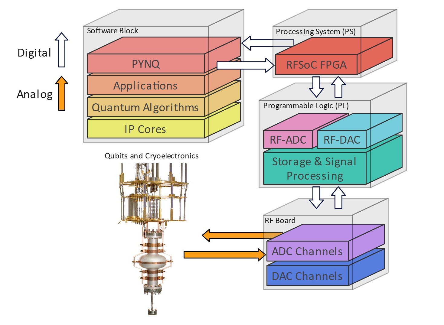
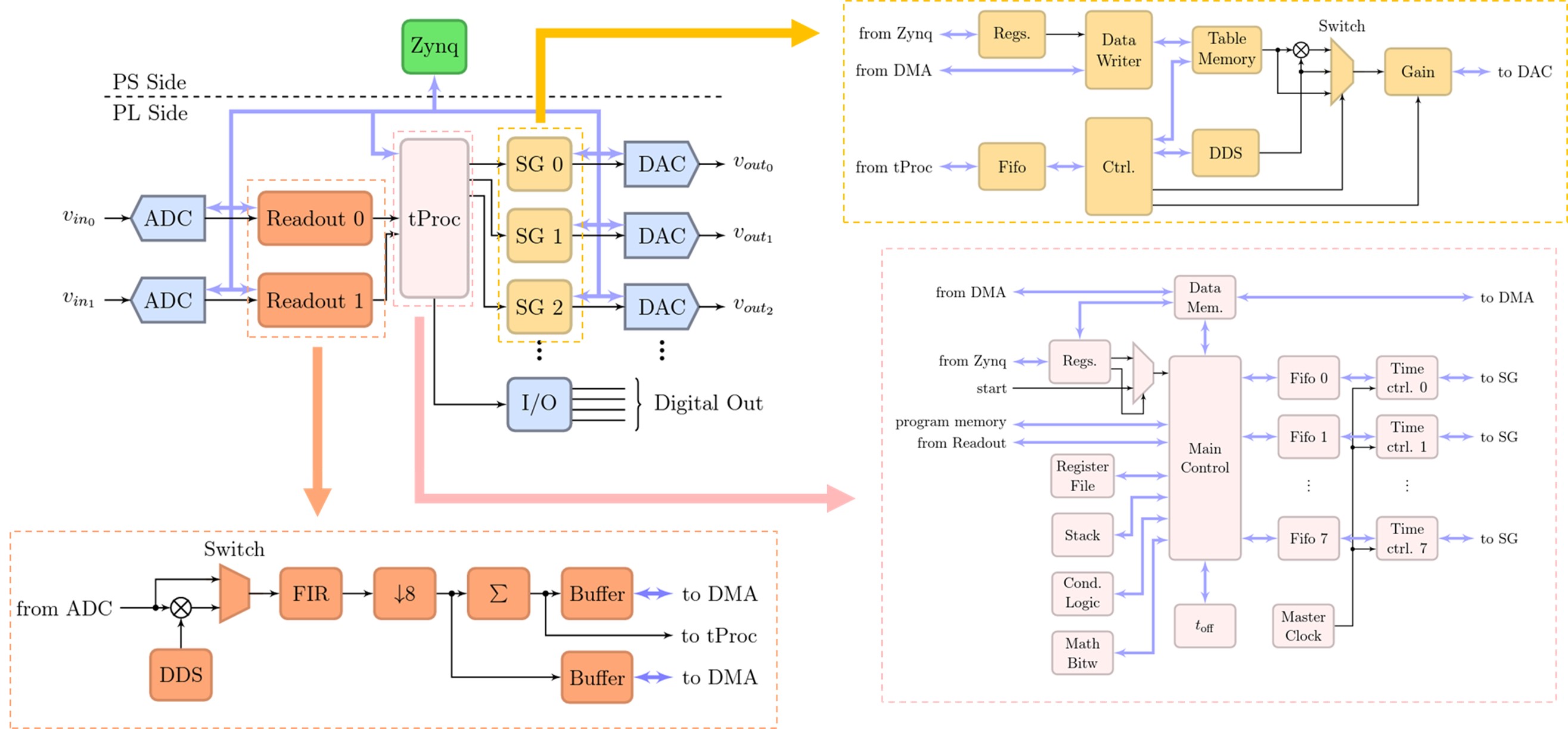
6. Control Electronics: The QICK Platform
The Quantum Instrumentation Control Kit (QICK) is an open-source qubit control platform developed at Fermilab [14]. It provides the classical electronics interface for superconducting quantum computers, representing a paradigm shift from traditional rack-mounted instrumentation to integrated FPGA-based control.
6.1 System Architecture
TABLE IX: QICK RFSoC Components
| Component |
Specification |
Function |
| RF DACs |
Up to 9.85 GSPS, 14-bit |
Direct synthesis of control pulses up to 6 GHz |
| RF ADCs |
Up to 4.096 GSPS, 12-bit |
Digitize readout signals |
| Programmable Logic |
~900K logic cells |
Real-time signal processing, tProcessor |
| ARM Processors |
Quad-core Cortex-A53 |
Python interface, experiment control |
Why FPGAs Instead of Traditional Instrumentation?
Traditional qubit control systems rely on stacks of commercial arbitrary waveform generators (AWGs), local oscillators, mixers, and digitizers—often filling entire equipment racks for a single qubit [15]. This approach has several limitations:
- Cost: Commercial AWGs capable of direct microwave synthesis cost $50,000-$200,000 per channel
- Synchronization: Coordinating timing across multiple instruments introduces jitter and complexity
- Latency: Communication between rack instruments and control computers adds microseconds of delay
- Scalability: Adding qubits requires proportionally more equipment
RFSoC FPGAs address these challenges by integrating high-speed data converters directly with programmable logic on a single chip.
6.2 QICK Firmware Architecture
The QICK firmware is built around three core components: the tProcessor (tProc) for timing control, the signal generator (SG) blocks for pulse synthesis, and the readout blocks for signal acquisition and processing.
Key Improvements in V2:
- RISC architecture: The 72-bit tProc V2 uses a pipelined RISC design, improving instruction throughput
- Polyphase filter bank: Enables simultaneous processing of up to 16 frequency-multiplexed readout channels
- Frequency-multiplexed output: Multiple tones can be generated on a single DAC channel
- Enhanced memory architecture: Separate memories with dual-port access for concurrent read/write
Key Insight: The evolution from QICK V1 to V2 reflects the scaling demands of quantum computing. V1's single-channel readout becomes a bottleneck when characterizing multi-qubit systems. V2's polyphase filter bank enables simultaneous readout of multiple qubits through frequency multiplexing.
6.3 The tProcessor: Timing and Synchronization
The tProcessor (timed processor) is QICK's solution for deterministic, cycle-accurate control:
EE Analogy: The tProcessor is like a hardware sequencer with absolute timestamping. Every pulse and acquisition has a precise timestamp relative to a master clock, eliminating software-induced jitter.
Music Analogy: The tProcessor is like an orchestra conductor who keeps every musician in perfect sync. Without the conductor, the violins might rush, the brass might drag, and the piece falls apart. The tProcessor ensures every control pulse hits at exactly the right moment.
TABLE X: QICK tProcessor Timing Specifications
| Parameter |
Value |
Significance |
| Timing jitter |
<2 ps RMS |
Negligible compared to qubit timescales |
| Total latency |
184-211 ns |
Deterministic, not variable |
| Instruction execution |
Timed instructions |
Events occur at absolute timestamps |
| Multi-board sync |
<100 ps alignment |
Enables scaling beyond single board |
7. The Current State of Quantum Computing
7.1 NISQ, FTQC, and FASQ
TABLE XI: Quantum Computing Eras [16]
| Era |
Full Name |
Characteristics |
Status |
| NISQ |
Noisy Intermediate-Scale Quantum |
50-1000 qubits, no QEC, limited depth |
Current |
| FTQC |
Fault-Tolerant QC |
Error-corrected logical qubits |
Early demos |
| FASQ |
Fault-tolerant Application-Scale |
Useful error-corrected computation |
Future goal |
7.2 The Error Budget
TABLE XII: Quantum Computing Error Budget
| Error Source |
Typical Rate |
Trend |
| Two-qubit gates |
0.1-1% |
Improving with better calibration |
| Single-qubit gates |
0.01-0.1% |
Approaching physical limits |
| Readout |
0.5-5% |
Major bottleneck |
| State preparation |
0.1-1% |
Limited by thermal population |
| Idle error (per μs) |
0.01-0.1% |
T1, T2 improvements ongoing |
7.3 Why Readout Matters for Error Correction
Quantum error correction (QEC) works by encoding a single logical qubit in many physical qubits and repeatedly measuring "syndrome" qubits to detect errors. For the surface code:
- Syndrome measurements must complete in ~1 μs (before errors accumulate)
- Each syndrome measurement requires single-shot readout
- Readout errors can be mistaken for data errors, causing incorrect corrections
- The error correction threshold requires physical error rates below ~1%
8. Qubit Performance Metrics and Platform Comparison
8.1 Key Qubit Metrics
T1: Energy Relaxation Time
T1 measures how long a qubit remains in the excited state \(|1\rangle\) before spontaneously decaying to the ground state \(|0\rangle\):
\[P_{|1\rangle}(t) = P_{|1\rangle}(0) \cdot e^{-t/T_1}\]
(19)
EE Analogy: T1 is the quantum equivalent of a capacitor's discharge time constant. Just as a charged capacitor loses energy to its environment through resistive losses, an excited qubit loses energy through various dissipation mechanisms.
Music Analogy: T1 is like how long a guitar string keeps ringing after you pluck it. A high-quality guitar in a quiet room rings for a long time; a cheap guitar in a noisy room dies out quickly.
T2: Dephasing (Coherence) Time
T2 measures how long a qubit maintains phase coherence in a superposition state:
\[T_2 \leq 2T_1 \quad \text{(fundamental limit)}\]
(20)
EE Analogy: T2 is analogous to phase noise in an oscillator. A qubit in superposition acts like a quantum oscillator; T2 measures how long the "clock" stays synchronized before environmental noise causes the phase to drift unpredictably.
Music Analogy: T2 is like how long an orchestra can play without a conductor before the musicians drift out of sync. At first, everyone is perfectly together. But over time, tiny timing differences accumulate until the ensemble falls apart.
Rabi Oscillation and Gate Time:
\[|\psi(t)\rangle = \cos\left(\frac{\Omega_R t}{2}\right)|0\rangle - i\sin\left(\frac{\Omega_R t}{2}\right)|1\rangle\]
(21)
Gate Fidelity:
\[F = \left\langle \psi \left| U^\dagger \mathcal{E}(|\psi\rangle\langle\psi|) U \right| \psi \right\rangle\]
(22)
Key Insight: Raw coherence time is less important than the number of operations achievable within T2. A platform with T2 = 100 μs and 50 ns gates can perform ~2000 operations before decoherence dominates. The relevant figure of merit is:
\[N_{\text{ops}} = \frac{T_2}{t_{\text{gate}}}\]
(23)
Quantitative Scaling Example:
\[F_{\text{circuit}} \approx (1 - \epsilon_{1Q})^{n \cdot d_{1Q}} \cdot (1 - \epsilon_{2Q})^{n_{\text{2Q gates}}} \cdot (1 - \epsilon_{\text{readout}})^{n}\]
(24)
The Scaling Wall: This exponential decay of fidelity with circuit size is why quantum error correction is essential. Without it, useful quantum computations on 100+ qubits are impossible with current error rates.
8.2 Quantum Computing Platform Comparison
TABLE XIII: Quantum Computing Platform Comparison
| Platform |
T1 |
T2 |
1Q Gate |
2Q Fidelity |
Max Qubits |
| Supercond. (Industry) [29,30,31] |
50-200 μs |
50-150 μs |
20-50 ns |
99.0-99.5% |
1,121 (IBM) |
| Supercond. (Lab best) [28] |
1.6 ms |
~1 ms |
20-50 ns |
99.5% |
6 (Princeton) |
| SQMS (Fermilab) [27,44] |
0.6 ms |
0.3 ms |
20-50 ns |
~99% |
9 (Rigetti) |
| SQMS 3D SRF [43,45] |
>2 s |
>20 ms |
~100 ns |
~99% |
2 qudits |
| Trapped Ions [32,33,34,35] |
>10 s |
1-10 s |
1-10 μs |
99.9-99.99% |
56 (H2) |
| Neutral Atoms [36,37] |
119 s |
12.6 s |
0.1-1 μs |
99.0-99.5% |
6,100 |
| Silicon Spin [38,39,40] |
9.5 s |
1.9 ms |
1-10 μs |
>99% |
~10 |
| Photonic [41,42] |
N/A |
Limited |
~ps |
~99.2% |
216+ modes |
8.3 SQMS Contributions to Coherence
The Superconducting Quantum Materials and Systems (SQMS) Center at Fermilab has made significant contributions to extending qubit coherence through materials science innovations [27]:
Surface Encapsulation Technique: SQMS researchers identified the niobium surface oxide as the primary source of energy loss in transmon qubits. Their surface encapsulation technique prevents the formation of lossy niobium oxide.
3D SRF Cavity Architecture: SQMS leverages Fermilab's expertise in superconducting radio-frequency (SRF) cavities from particle accelerator development:
- Cavity photon lifetimes exceeding 2 seconds demonstrated
- Two-qudit QPU with >20 ms coherence (record for multimode superconducting system)
- Qudit encoding: single cavity stores multiple quantum levels
\[\mathcal{D}_{\text{qudit}} = d^n\]
(25)
\[N_{\text{eff}} = n \cdot \log_2(d)\]
(26)
SQMS Vision: The Center aims to achieve 10 ms coherence in chip-based transmon qubits and deploy a 100+ qudit SRF quantum processor (equivalent to ~500 qubits in computational space) within a single dilution refrigerator.
9. Application: Adaptive Filtering for Qubit Readout
This section describes how adaptive Wiener filtering [19,20] can address the readout bottleneck described in previous sections.
9.1 The Filtering Approach
TABLE XIV: Comparison of Filtering Approaches
| Approach |
Advantages |
Disadvantages |
| Ensemble averaging |
Simple, no training needed |
Requires N experiments, incompatible with single-shot |
| Fixed matched filter |
Optimal for known statistics |
Must re-derive if system changes |
| Adaptive filter |
Learns from data, adapts to drift |
Requires training phase |
9.2 Training and Inference
Training Phase:
- Prepare qubit in \(|0\rangle\) (ground state, by waiting for T1 decay)
- Collect many readout pulses → label as class "0"
- Apply \(\pi\)-pulse to prepare \(|1\rangle\)
- Collect many readout pulses → label as class "1"
- LMS algorithm iteratively adjusts filter weights to minimize classification error
Inference Phase:
- Freeze filter weights (no further adaptation)
- For each readout pulse, apply fixed weights
- Output is a single (I, Q) point with improved SNR
- Classify based on decision boundary
9.3 Performance Summary
TABLE XV: Adaptive Filter Performance Summary
| Metric |
Value |
Significance |
| SNR improvement |
+9 dB (64 taps) |
Equivalent to 64× averaging |
| Latency |
<1 μs |
Compatible with QEC timing |
| Training time |
~1000 pulses |
Practical for calibration routines |
| Implementation |
FPGA (QICK-compatible) |
Real-time, no software latency |
Validation Status: The performance metrics above have been verified through RTL simulation on FPGA using synthetic Gaussian noise models. Hardware validation with actual superconducting qubit readout signals is currently in progress.
10. Mathematical Foundations (Reference)
This section collects the key mathematical results for readers seeking deeper understanding. It can be skipped without loss of continuity.
The transmon Hamiltonian in the phase basis:
\[\hat{H} = 4E_C(\hat{n} - n_g)^2 - E_J\cos\hat{\phi} \tag{27}\]
In the transmon regime (\(E_J/E_C \gg 1\)), the energy levels are approximately:
\[E_m \approx -E_J + \sqrt{8E_JE_C}\left(m + \frac{1}{2}\right) - \frac{E_C}{12}(6m^2 + 6m + 3) \tag{28}\]
The transition frequencies are:
\[\hbar\omega_{01} \approx \sqrt{8E_JE_C} - E_C, \quad \alpha = \omega_{01} - \omega_{12} \approx -E_C/\hbar \tag{29}\]
The qubit-resonator system in the dispersive regime:
\[\hat{H}_{\text{disp}} = \hbar\omega_r\hat{a}^\dagger\hat{a} + \frac{\hbar\omega_q}{2}\hat{\sigma}_z + \hbar\chi\hat{a}^\dagger\hat{a}\hat{\sigma}_z \tag{30}\]
The dispersive shift is:
\[\chi = \frac{g^2}{\Delta}\frac{\alpha}{\Delta + \alpha} \tag{31}\]
The resonator frequency conditioned on qubit state:
\[\omega_r^{|0\rangle} = \omega_r + \chi, \quad \omega_r^{|1\rangle} = \omega_r - \chi \tag{32}\]
The Wiener filter minimizes mean-squared error:
\[\mathbf{w}_{\text{opt}} = \mathbf{R}_{xx}^{-1}\mathbf{r}_{xd} \tag{33}\]
For white noise and a known signal template, the optimal gain is:
\[G_{\text{opt}} = \frac{\text{SNR}}{1 + \text{SNR}} = \frac{P_{\text{signal}}}{P_{\text{signal}} + P_{\text{noise}}} \tag{34}\]
The SNR improvement from an \(N_t\)-tap filter:
\[\text{SNR}_{\text{out}} = \text{SNR}_{\text{in}} + 10\log_{10}(N_t) \text{ dB} \tag{35}\]
The Least Mean Squares (LMS) algorithm [20] updates weights iteratively:
\[\mathbf{w}[n+1] = \mathbf{w}[n] + \mu \cdot e^*[n] \cdot \mathbf{x}[n] \tag{36}\]
where \(\mu\) = step size (learning rate), \(e[n] = d[n] - y[n]\) = error signal, and \(y[n] = \mathbf{w}^H[n]\mathbf{x}[n]\) = filter output.
The Block NLMS variant normalizes by input power:
\[\mathbf{w}[n+1] = \mathbf{w}[n] + \frac{\mu}{\|\mathbf{x}\|^2 + \epsilon} \cdot e^*[n] \cdot \mathbf{x}[n] \tag{37}\]
11. Conclusion
Superconducting quantum computing, despite its quantum mechanical foundations, is largely an electrical engineering endeavor. The qubit is a nonlinear LC oscillator; control and readout involve RF pulse generation and detection; and improving performance requires signal processing techniques familiar to any EE.
The readout bottleneck, in particular, is a classic signal processing problem: discriminating two Gaussian-distributed classes in the presence of noise. Adaptive filtering techniques, long used in communications and radar, can provide significant improvements in single-shot readout fidelity, directly enabling quantum error correction.
Summary of Key Points:
- A transmon qubit is a Josephson junction shunted by a capacitor, forming a nonlinear LC oscillator
- The Josephson junction acts as a current-dependent inductor: \(L_J = \Phi_0/(2\pi I_c \cos\delta)\)
- Nonlinearity creates anharmonic energy levels, enabling selective \(|0\rangle\leftrightarrow|1\rangle\) addressing
- Dispersive readout measures state-dependent resonator frequency shift (~1-5 MHz)
- Single-shot readout is required for QEC; ensemble averaging is not sufficient
- Optimal filtering can achieve the same SNR improvement as averaging, in a single shot
- QICK provides deterministic timing (<2 ps jitter) for coherent control
- Readout error (0.5-5%) is currently a major bottleneck; improving it enables QEC
For detailed treatment of the adaptive Wiener filter implementation, see the companion document: "Block NLMS Adaptive Wiener Filter for Superconducting Qubit Readout."
References
[1] P. W. Shor, "Algorithms for quantum computation: Discrete logarithms and factoring," Proc. 35th Annual Symposium on Foundations of Computer Science, pp. 124-134, 1994.
[2] L. K. Grover, "A fast quantum mechanical algorithm for database search," Proc. 28th Annual ACM Symposium on Theory of Computing, pp. 212-219, 1996.
[3] A. W. Harrow, A. Hassidim, and S. Lloyd, "Quantum algorithm for linear systems of equations," Physical Review Letters, vol. 103, p. 150502, 2009.
[4] B. D. Josephson, "Possible new effects in superconductive tunnelling," Physics Letters, vol. 1, no. 7, pp. 251-253, 1962.
[5] L. N. Cooper, "Bound electron pairs in a degenerate Fermi gas," Physical Review, vol. 104, no. 4, pp. 1189-1190, 1956.
[6] J. Bardeen, L. N. Cooper, and J. R. Schrieffer, "Theory of superconductivity," Physical Review, vol. 108, no. 5, pp. 1175-1204, 1957.
[7] M. A. Nielsen and I. L. Chuang, Quantum Computation and Quantum Information, 10th Anniversary ed. Cambridge University Press, 2010.
[8] D. J. Griffiths, Introduction to Quantum Mechanics, 3rd ed. Cambridge University Press, 2018.
[9] M. H. Devoret and R. J. Schoelkopf, "Superconducting circuits for quantum information: An outlook," Science, vol. 339, pp. 1169-1174, 2013.
[10] J. Koch et al., "Charge-insensitive qubit design derived from the Cooper pair box," Physical Review A, vol. 76, no. 4, p. 042319, 2007.
[11] A. G. Fowler, M. Mariantoni, J. M. Martinis, and A. N. Cleland, "Surface codes: Towards practical large-scale quantum computation," Physical Review A, vol. 86, no. 3, p. 032324, 2012.
[12] A. Blais, A. L. Grimsmo, S. M. Girvin, and A. Wallraff, "Circuit quantum electrodynamics," Reviews of Modern Physics, vol. 93, no. 2, p. 025005, 2021.
[13] T. Walter et al., "Rapid high-fidelity single-shot dispersive readout of superconducting qubits," Physical Review Applied, vol. 7, no. 5, p. 054020, 2017.
[14] L. Stefanazzi et al., "The QICK (Quantum Instrumentation Control Kit): Readout and control for qubits and detectors," Review of Scientific Instruments, vol. 93, no. 4, p. 044709, 2022.
[15] P. Krantz et al., "A quantum engineer's guide to superconducting qubits," Applied Physics Reviews, vol. 6, no. 2, p. 021318, 2019.
[16] J. Preskill, "Quantum Computing in the NISQ era and beyond," Quantum, vol. 2, p. 79, 2018.
[17] J. Preskill, "Beyond NISQ: The Megaquop Machine," Keynote address at Q2B 2024 Conference, December 2024.
[18] J. Eisert and J. Preskill, "The quantum computing bubble," arXiv:2411.03528, November 2025.
[19] S. Haykin, Adaptive Filter Theory, 5th ed. Upper Saddle River, NJ: Pearson, 2014.
[20] B. Widrow and S. D. Stearns, Adaptive Signal Processing. Englewood Cliffs, NJ: Prentice-Hall, 1985.
[21] M. A. Rol et al., "Restless Tuneup of High-Fidelity Qubit Gates," Physical Review Applied, vol. 7, p. 041001, 2017.
[22] S. Sheldon et al., "Characterizing errors on qubit operations via iterative randomized benchmarking," Physical Review A, vol. 93, p. 012301, 2016.
[23] J. M. Gambetta, J. M. Chow, and M. Steffen, "Building logical qubits in a superconducting quantum computing system," npj Quantum Information, vol. 3, p. 2, 2017.
[24] C. Müller, J. H. Cole, and J. Lisenfeld, "Towards understanding two-level-systems in amorphous solids: Insights from quantum circuits," Reports on Progress in Physics, vol. 82, p. 124501, 2019.
[25] J. Kelly et al., "State preservation by repetitive error detection in a superconducting quantum circuit," Nature, vol. 519, pp. 66-69, 2015.
[26] D. C. McKay et al., "Universal Gate for Fixed-Frequency Qubits via a Tunable Bus," Physical Review Applied, vol. 6, p. 064007, 2016.
[27] M. Bal et al., "Systematic improvements in transmon qubit coherence enabled by niobium surface encapsulation," npj Quantum Information, vol. 10, p. 43, 2024.
[28] F. Bahrami et al., "High-coherence transmon qubits on tantalum-on-silicon," Nature, November 2025. (Princeton T1 > 1.6 ms result)
[29] Google Quantum AI, "Quantum error correction below the surface code threshold," Nature, December 2024. (Willow processor)
[30] IBM Quantum, "IBM Launches Its Most Advanced Quantum Computers," IBM Newsroom, November 2024. (Heron R2: 156 qubits)
[31] Y. Kim et al., "Evidence for the utility of quantum computing before fault tolerance," Nature, vol. 618, pp. 500-505, 2023.
[32] Quantinuum, "Quantinuum extends its significant lead in quantum computing," Quantinuum Blog, April 2024. (H1: 99.914% 2Q gate fidelity)
[33] Quantinuum, "Quantinuum's H-Series hits 56 physical qubits," Quantinuum Blog, June 2024.
[34] P. Wang et al., "Single ion qubit with estimated coherence time exceeding one hour," Nature Communications, vol. 12, p. 233, 2021.
[35] C. Monroe et al., "Progress in Trapped-Ion Quantum Simulation," Annual Review of Condensed Matter Physics, vol. 16, pp. 145-172, 2025.
[36] H. Levine et al., "A tweezer array with 6,100 highly coherent atomic qubits," Nature, September 2025.
[37] S. J. Evered et al., "High-fidelity parallel entangling gates on a neutral-atom quantum computer," Nature, vol. 622, pp. 268-272, 2023.
[38] N. Samkharadze et al., "Industry-compatible silicon spin-qubit unit cells exceeding 99% fidelity," Nature, vol. 646, pp. 81-87, September 2025.
[39] B. Sun et al., "Full-Permutation Dynamical Decoupling in Triple-Quantum-Dot Spin Qubits," PRX Quantum, vol. 5, p. 020356, 2024.
[40] S. D. Ha et al., "Two-dimensional Si spin qubit arrays with multilevel interconnects," PRX Quantum, vol. 6, p. 030327, 2025.
[41] PsiQuantum, "Omega: A manufacturable chipset for photonic quantum computing," Nature, February 2025.
[42] Xanadu, "On-chip generation of GKP states for fault-tolerant quantum computing," Nature, June 2025.
[43] T. Roy et al., "Qudit-based quantum computing with SRF cavities at Fermilab," FERMILAB-CONF-24-0026-SQMS, 2024.
[44] SQMS Center, "Researchers achieve leading performance in transmon qubits," Fermilab News, May 2024.
[45] SQMS Center, "Fermilab's SQMS Center funded with $125 million," Fermilab News, November 2025.
[46] J. Van Damme et al., "Advanced CMOS manufacturing of superconducting qubits on 300 mm wafers," Nature, September 2024.
[47] T. E. Roth, R. Ma, and W. C. Chew, "The Transmon Qubit for Electromagnetics Engineers: An Introduction," IEEE Antennas and Propagation Magazine, vol. 65, no. 2, April 2023.
[48] The Quantum Insider, "What Is The Price Of A Quantum Computer In 2025?," December 2025.